하이퍼파라미터튜닝
-그리드서치
-아웃라이어
배깅(Bagging)
보팅(voting)
그리드서치(GridSearchCV)
- 하이퍼파라미터 튜닝: 임의의 값들을 넣어 더 나은 결과를 찾는 방식 ->수정 및 재시도하는 단순 작업의 반복
- 그리드 서치: 수백가지 하이퍼파라미터값을 한 번에 적용가능
- 그리드서치의 원리: 입력할 하이퍼파라미터 후보들을 입력한 후, 각 조합에 대해 모두 모델링해보고 최적의 결과가 나오는 하이퍼파라미터 조합을 확인
param = [
    {'n_estimators' : [100, 200], 'max_depth':[6, 8, 10, 12], 'n_jobs' : [-1, 2, 4]},
    {'max_depth' : [6, 8, 10, 12], 'min_samples_split' : [2, 3, 5, 10]},
    {'n_estimators' : [100, 200], 'min_samples_leaf' : [3, 5, 7, 10]},
    {'min_samples_split' : [2, 3, 5, 10], 'n_jobs' : [-1, 2, 4]},
    {'n_estimators' : [100, 200],'n_jobs' : [-1, 2, 4]}
	]

#2. 모델
from sklearn.model_selection import GridSearchCV
rf_model = RandomForestClassifier()
model = GridSearchCV(rf_model, param, cv=kfold, verbose=1,
                     refit=True, n_jobs=-1) #refit 기본값은 False라 꼭 True로 해줘야함: 위에 입력한 파라미터를 찾아서 적용하는 기능

#3. 훈련
import time
start_time = time.time()
model.fit(x_train, y_train)
end_time= time.time() - start_time

print('최적의 파라미터 : ' , model.best_params_)
print('최적의 매개변수 : ' , model.best_estimator_)
print('best_score : ', model.best_score_)
print('model_score : ', model.score(x_test, y_test))
print('걸린 시간 : ', end_time, '초')
결과값
최적의 파라미터 :  {'min_samples_leaf': 10, 'n_estimators': 200}
최적의 매개변수 :  RandomForestClassifier(min_samples_leaf=10, n_estimators=200)
best_score :  0.9583333333333334
model_score :  1.0
걸린 시간 :  10.046573162078857 초
최적의 파라미터 값 확인 후 모델 수정하기
#2. 모델
from sklearn.model_selection import GridSearchCV
model = RandomForestClassifier(max_depth=6, n_estimators= 200, n_jobs= -1)
그리드 값을 랜덤으로 구할 수도 있다.
RandomForestRegressor
param 설정 후

#2. 모델
from sklearn.model_selection import GridSearchCV
rf_model = RandomForestRegressor()
model = GridSearchCV(rf_model, param, cv=kfold, verbose=1,
                     refit=True, n_jobs=-1)
1. XGBoost 모델의 parameters
'n_estimators': [100,200,300,400,500,1000]} #default 100 / 1~inf(무한대) / 정수
'learning_rate' : [0.1, 0.2, 0.3, 0.5, 1, 0.01, 0.001] #default 0.3/ 0~1 / learning_rate는 eta라고 해도 적용됨
'max_depth' : [None, 2,3,4,5,6,7,8,9,10] #default 3/ 0~inf(무한대) / 정수 => 소수점은 정수로 변환하여 적용해야 함
'gamma': [0,1,2,3,4,5,7,10,100] #default 0 / 0~inf
'min_child_weight': [0,0.01,0.01,0.1,0.5,1,5,10,100] #default 1 / 0~inf
'subsample' : [0,0.1,0.2,0.3,0.5,0.7,1] #default 1 / 0~1
'colsample_bytree' : [0,0.1,0.2,0.3,0.5,0.7,1] #default 1 / 0~1
'colsample_bylevel' : [0,0.1,0.2,0.3,0.5,0.7,1] #default 1 / 0~1
'colsample_bynode' : [0,0.1,0.2,0.3,0.5,0.7,1] #default 1 / 0~1
'reg_alpha' : [0, 0.1,0.01,0.001,1,2,10] #default 0 / 0~inf / L1 절대값 가중치 규제 / 그냥 alpha도 적용됨
'reg_lambda' : [0, 0.1,0.01,0.001,1,2,10] #default 1 / 0~inf / L2 제곱 가중치 규제 / 그냥 lambda도 적용됨
2. LightGBM 모델의 parameters
대체로 XGBoost와 하이퍼 파라미터들이 비슷하지만 leaf-wise 방식의 하이퍼 파라미터가 존재함
num_leaves : 하나의 트리가 가질 수 있는 최대 리프 개수
min_data_in_leaf : 오버피팅을 방지할 수 있는 파라미터, 큰 데이터셋에서는 100이나 1000 정도로 설정
feature_fraction : 트리를 학습할 때마다 선택하는 feature의 비율
n_estimators : 결정 트리 개수
learning_rate : 학습률
reg_lambda : L2 규제
reg_alpha : L1규제
max_depth : 트리 개수 제한
3. Catboost 모델의 parameters
CatBoost 평가 지표 최적화에 가장 큰 영향을 미치는 하이퍼파라미터는 learning_rate, depth, l2_leaf_reg 및
random_strength
learning_rate: 학습률
depth: 각 트리의 최대 깊이로 과적합을 제어
l2_leaf_reg: L2 정규화(regularization) 강도로, 과적합을 제어
colsample_bylevel: 각 트리 레벨에서의 피처 샘플링 비율
n_estimators: 생성할 트리의 개수
subsample: 각 트리를 학습할 때 사용할 샘플링 비율
border_count: 수치형 특성 처리 방법
ctr_border_count: 범주형 특성 처리 방법
아웃라이어(outliers)
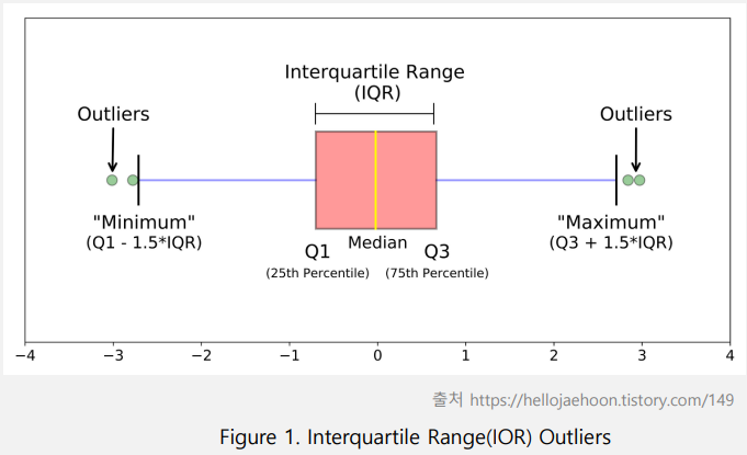
IQR은 사분위 값의 편차를 이용하여 이상치를 걸러내는 방법
전체 데이터를 정렬 후 4등분 - Q1(25%), Q2(50%), Q3(75%), Q4(100%)
IQR = Q3 - Q1
예제)
import numpy as np

oliers = np.array([-50,-10,2,3,4,5,6,7,8,9,10,11,12,50])

def outliers (data_out):
    quartile_1, q2, quartile_3 = np.percentile(data_out,
                                              [25,50,75])       #등분하는거
    print('1사분위 : ', quartile_1)
    print('2사분위 : ', q2)
    print('3사분위 : ', quartile_3)

    iqr = quartile_3 - quartile_1
    print('IQR : ',iqr)

    lower_bound = quartile_1 - (iqr*1.5)    #낮은 이상치
    upper_bound = quartile_3 + (iqr*1.5)    #높은 이상치
    print('lower_bound : ', lower_bound)
    print('upper_bound : ', upper_bound)
    return np.where((data_out>upper_bound) |
                    (data_out<lower_bound))

outliers_loc = outliers(oliers)
print('이상치의 위치 : ', outliers_loc)
***********
1사분위 :  3.25
2사분위 :  6.5
3사분위 :  9.75
IQR :  6.5
lower_bound :  -6.5
upper_bound :  19.5
이상치의 위치 :  (array([ 0,  1, 13], dtype=int64),)
#시각화
import matplotlib.pyplot as plt
plt.boxplot(oliers)
plt.show()
=> 컬럼 별로 이상치 확인 후 제거하는 전처리 작업을 해야한다.
배깅(Bagging)
샘플을 여러번 뽑아 각 모델을 학습시켜 결과물을 집계하는 방법(BaggingClassifier, BaggingRegressor)
from sklearn.ensemble import BaggingRegressor


#2. 모델(Bagging)
bagging = BaggingRegressor(DecisionTreeRegressor(),
                            n_estimators=100,
                            n_jobs=-1,
                            random_state=42)

#3. 훈련
start_time = time.time()
bagging.fit(x_train,y_train)
end_time = time.time() - start_time

#4. 평가,예측
result = bagging.score(x_test,y_test)

print('걸린시간: ', end_time, '초')
print('bagging 결과 : ', result)
배깅 + scaler, kfold, grid
from sklearn.ensemble import BaggingRegressor

# 스케일러
scaler = MinMaxScaler()
x_train = scaler.fit_transform(x_train)
x_test = scaler.transform(x_test)

#KFold
n_split = 5
kfold = KFold(n_splits=n_split, shuffle=True, random_state=42)

#parameter
param ={
    'n_estimators': [100],
    'random_state':[42,62,72],
    'max_features':[3,4,7]
}

#2. 모델(Bagging)
bagging = BaggingRegressor(DecisionTreeRegressor(),
                            n_estimators=100,
                            n_jobs=-1,
                            random_state=42)
model = GridSearchCV(bagging, param, cv=kfold, refit=True, n_jobs=-1)

#3. 훈련
start_time = time.time()
model.fit(x_train,y_train)
end_time = time.time() - start_time

#4. 평가,예측
result = model.score(x_test,y_test)

print('최적의 매개변수 : ', model.best_estimator_)
print('최적의 파라미터 : ', model.best_params_)
print('걸린시간: ', end_time, '초')
print('bagging 결과 : ', result)
보팅(Voting)
서로 다른 알고리즘을 가진 분류기를 결합하는 것
하드보팅: 각 분류기의 예측결과를 다수결로 결정
소프트보팅: 각 분류기의 예측 확률을 평균하여 예측을 수행
VotingRegressor/VotingClassifier
#2. 모델(voting)
xgb = XGBClassifier()
lgbm = LGBMClassifier()
cat = CatBoostClassifier()

model = VotingClassifier(estimators=[('xgb', xgb),('lgbm', lgbm),('cat', cat)],# 모델이랑 이름 같이 넣어줘야함
                         voting = 'hard',
                         n_jobs=-1)

#3. 훈련
model.fit(x_train,y_train)

***********
정확도 확인
classifiers = [cat,xgb,lgbm,]
for model in classifiers:
    model.fit(x_train,y_train)
    y_predict=model.predict(x_test)
    score = accuracy_score(y_test, y_predict)
    class_name = model.__class__.__name__
print('{0} 정확도: {1: .4f}'.format(class_name, score))'[네이버클라우드] 클라우드 기반의 개발자 과정 7기 > AI' 카테고리의 다른 글
| [수업자료] ml2 오늘의 코드 -gridsearch, random, bagging (0) | 2023.05.16 |
|---|---|
| [수업자료] ml1 오늘의 코드3 (0) | 2023.05.16 |
| 머신러닝 1 / feature importance (0) | 2023.05.16 |
| 머신러닝 1 -model, scaling (0) | 2023.05.15 |
| heatmap NaN, label Encoding - 팀플 쓰기 (2) | 2023.05.12 |